Lack-of-fit sum of squares
In statistics, a sum of squares due to lack of fit, or more tersely a lack-of-fit sum of squares, is one of the components of a partition of the sum of squares in an analysis of variance, used in the numerator in an F-test of the null hypothesis that says that a proposed model fits well.
Contents |
Sketch of the idea
In order to have a lack-of-fit sum of squares one observes more than one value of the response variable for each value of the set of predictor variables. For example, consider fitting a line
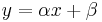
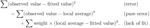
by the method of least squares. One takes as estimates of α and β the values that minimize the sum of squares of residuals, i.e., the sum of squares of the differences between the observed y-value and the fitted y-value. To have a lack-of-fit sum of squares, one observes more than one y-value for each x-value. One then partitions the "sum of squares due to error", i.e., the sum of squares of residuals, into two components:
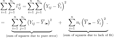
- sum of squares due to error = (sum of squares due to "pure" error) + (sum of squares due to lack of fit).
The sum of squares due to "pure" error is the sum of squares of the differences between each observed y-value and the average of all y-values corresponding to the same x-value.
The sum of squares due to lack of fit is the weighted sum of squares of differences between each average of y-values corresponding to the same x-value and corresponding fitted y-value, the weight in each case being simply the number of observed y-values for that x-value.[1][2]
In order that these two sums be equal, it is necessary that the vector whose components are "pure errors" and the vector of lack-of-fit components be orthogonal to each other, and one may check that they are orthogonal by doing some algebra.
Mathematical details
Consider fitting a line, where i is an index of each unique x value, and j is an index of an observation for a given x value. The value of each observation can be represented by

Let

be the least squares estimates of the unobservable parameters α and β based on the observed values of x i and Y i j.
Let
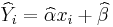
be the fitted values of the response variable. Then
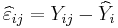
are the residuals, which are observable estimates of the unobservable values of the error term ε ij. Because of the nature of the method of least squares, the whole vector of residuals, with

scalar components, necessarily satisfies the two constraints
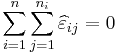
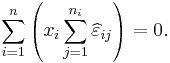
It is thus constrained to lie in an (N − 2)-dimensional subspace of R N, i.e. there are N − 2 "degrees of freedom for error".
Now let
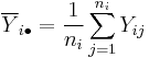
be the average of all Y-values associated with a particular x-value.
We partition the sum of squares due to error into two components:
Probability distributions
Sums of squares
Suppose the error terms ε i j are independent and normally distributed with expected value 0 and variance σ2. We treat x i as constant rather than random. Then the response variables Y i j are random only because the errors ε i j are random.
It can be shown to follow that if the straight-line model is correct, then the sum of squares due to error divided by the error variance,
has a chi-squared distribution with N − 2 degrees of freedom.
Moreover:
- The sum of squares due to pure error, divided by the error variance σ2, has a chi-squared distribution with N − n degrees of freedom;
- The sum of squares due to lack of fit, divided by the error variance σ2, has a chi-squared distribution with n − 2 degrees of freedom;
- The two sums of squares are probabilistically independent.
The test statistic
It then follows that the statistic
![\begin{align}
F & = \frac{ \text{lack-of-fit sum of squares} /\text{degrees of freedom} }{\text{pure-error sum of squares} / \text{degrees of freedom} } \\[8pt]
& = \frac{\left.\sum_{i=1}^n n_i \left( \overline Y_{i\bullet} - \widehat Y_i \right)^2\right/ (n-2)}{\left.\sum_{i=1}^n \sum_{j=1}^{n_i} \left(Y_{ij} - \overline Y_{i\bullet}\right)^2 \right/ (N - n)}
\end{align}](/2012-wikipedia_en_all_nopic_01_2012/I/fda3720797cac25837f312a4c4b1ad98.png)
has an F-distribution with the corresponding number of degrees of freedom in the numerator and the denominator, provided that the straight-line model is correct. If the model is wrong, then the probability distribution of the denominator is still as stated above, and the numerator and denominator are still independent. But the numerator then has a noncentral chi-squared distribution, and consequently the quotient as a whole has a non-central F-distribution.
One uses this F-statistic to test the null hypothesis that the straight-line model is right. Since the non-central F-distribution is stochastically larger than the (central) F-distribution, one rejects the null hypothesis if the F-statistic is too big. How big is too big—the critical value—depends on the level of the test and is a percentage point of the F-distribution.
The assumptions of normal distribution of errors and statistical independence can be shown to entail that this lack-of-fit test is the likelihood-ratio test of this null hypothesis.